수행기록

[GA] Quest 6 STM32Cube.AI와 B-L475E-IOT01A 보드를 이용하여 본인만의 AI 프로젝트 만들기 - 사각지대 지각을 위한 음향 장면 인식 프로젝트

2022. 9. 26 (월) 23:10 최종수정 2022. 10. 23 (일) 20:51 칩헤드 조회 4708 좋아요 2 스크랩 0 댓글 22

> 가속도 센서를 응용하시거나 (1) 다양한 센서의 데이터 로깅을 통해 STM32Cube.AI에서
> 지원가능한 상용 머신러닝툴을 사용하여 (2) Neural Network Model을 만들고
> (3) STM32Cube.AI로 변환한 C code Model를 적용한 (4) 어플리케이션을 자유롭게 만들어 보시면 됩니다.
>
> 1. 개발하신 어플리케이션이 B-L475E-IOT01A 보드에서 구동하는 동영상을 업로드 해주세요.
> 2. 상용 머신러닝 툴에서 사용한 Source Code를 업로드 해주세요.
> 3. B-L475E-IOT01A에 적용된 Application Source Code와 해당 Application에 대한 소개 및 설명을 포함하는 PDF 문서를 업로드하세요.
> (PDF 문서에는 2번의 머신러닝 툴에서의 Model에 대한 설명도 포함 합니다.
> 예를 들어 Model의 구성 설명이나 Accuracy 등과 같은 내용을 설명해 주시면 됩니다.)

Quest6 미션 과제의 수행 결과를 다음과 같이 포스팅합니다. IOT 개발보드를 이용하여 데이타의 학습 및 추론을 하면서
서버 및 데스크탑 PC와 달리 CPU/RAM 자원이 극히 제한된 임베디드 환경에서 알아야 할 주요 기술 지식들을
하나하나 정확이 이해를 하면서 피부로 경험할수 있는 더 없이 좋은 시간이었습니다. ^^

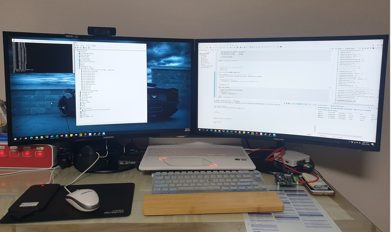
[B-L475E-IOT01A개발보드의 개발환경 셋업 화면]

- 다 음 -

(STM32Cube.AI와 B-L475E-IOT01A 보드를 이용한 ASC-AI 프로젝트)

Q6: 사각지대 지각을 위한 음향 장면 인식 프로젝트

참고) 아래의 목차중에서 해당 링크를 클릭하면 해당 부분으로 이동하도록 북마킹 되어 있습니다.

Data를 (.wav) 생성하기... 9

Data로 LogMel Spectrogram 생성... 12

LogMel Spectrogram으로 전처리 작업... 12

피쳐 표준화하기... 15

데이터 인코딩하기... 15

데이터셋을 훈련, 검증, 테스트 셋으로 분리... 16

Confusion Matrix 평가하기... 21

생성한 AI 모델 저장... 22

(선택사항) 양자화로 TFLite 모델 변환... 23

STM32.XCube AI 툴... 24

AI 모델을 C코드로 변환... 24

C 소스코드의 빌드 및 플래싱... 25

데모... 27

프로젝트 소개

이 섹션은 프로젝트의 목표 및 개발을 위한 환경 준비에 대한 내용을 설명합니다.

프로젝트 목표

저는 음향 이벤트 인식 기술은 오디오 신호에서 발생하는 이벤트 종류를 찾는 문제로, 최근 많은 연구가 이루어 지고 있습니다. 음향 장면 인식 기술은 시각적으로 확인할 수 없는 사각지대에 발생한 예상치 못한 상황을 소리만으로도 인식할 수 있습니다. 이 때문에 음향 장면 인식 기술을 활용하면 (1) 청력이 저하된 사람을 위한 공간 지각 서비스, (2) 안전 상황 감시, (3) 실내 상황 모니터링을 위한 AI 스피커 등 실생활에 매우 다양한 응용 기술의 개발이 가능합니다. 이러한 음향 장면 인식 기술의 발전을 위하여, 매년 IEEE 기관에서 DCASE Challenge (https://dcase.community/) 이라는 세계적인 인공지능 기반 음향 장면 인식 기술 대회가 개최할 정도로 미래 사회에서 중요한 기술들 중의 하나입니다.

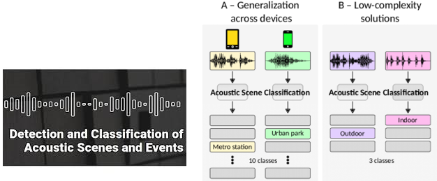
[DCASE Challenge 국제 대회의 ASC 입력 및 출력 방법 예시]

이번 자율 프로젝트에서는 ST IoT 개발보드와 STM32 Cube AI 툴을 이용하여 실내외 환경 및 차량내 환경에서 발생할 수 있는 다양한 소리들을 탐지하고 인공지능을 이용하여 더 똑똑하게 소리를 인식할 수 있는 음향 장면인식 프로젝트에 도전해보려고 합니다. 일반적으로 음성 인식은 음향 인식에 언어처리 부분을 추가합니다. 예를 들어, 음성입력 -> 특징 추출 -> 특징 벡터 -> 패턴 분류 -> 후보단위 -> 언어처리 -> 인식된 문장 이런 순서가 됩니다.

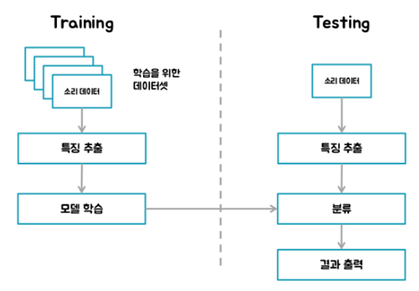
[소리 데이터의 학습 및 테스트 흐름도]

저는 딥러닝 기술을 이용하여 IoT 장치의 마이크가 캡처한 주변 소음을 분류할 수 있습니다. 이번 프로젝트에서는 행사 측에서 제공하는 IoT 개발보드에 내장되어 있는 마이크 장치를 이용하여 사운드를 입력 받고, 학습 후 AI모델을 만들 것입니다. 그리고나서 만든 AI모델을 C소스코드로 변환하고, 컴파일하여 펌웨어 이미지를 만들고, 이 펌웨어 이미지를 개발보드에 플래싱한 후에 음성 데이터가 Indoor음성인지, Outdoor음성인지, In-Vehicle 음성인지 분류하는 딥러닝 소프트웨어를 데모하려고 합니다.

제일 먼저 저는 사운드 입력을 3 가지 범주로 분류하기 위해 CNN이라는 딥러닝 모델을 생성해야 합니다. 다음 그림은 입력되는 음향 데이터들을 3개의 클래스로 분류후에 분류된 음향 데이터들을 학습하여 유사 음향 데이터가 입력으로 들어올 때 어떤 음향 데이터인지 인공지능을 통해 분류하는 작업을 위한 전체 개념도입니다.

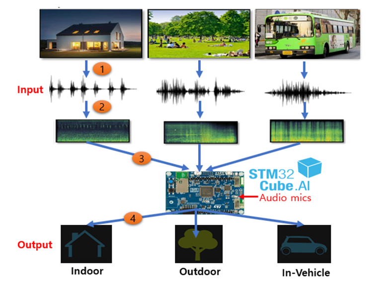
[음성 데이터를 Indoor, Outdoor, In-Vehicle으로 분류하기 위한 개념도]

Indoor (집안)
Outdoor (집밖)
In-Vehicle (차량내)

소프트웨어 준비

저는 수집한 음성 데이터들을 이용하여 모델 생성과 모델 학습을 달성하기 위하여 Keras소프트웨어를 사용할 것입니다. 그리고, 이 작업을 위하여 ST Microelectronics에 의해 제공되는 STM32용 FP-AI-SENSING1이라는 기본 패키지를 활용할 것입니다. IOT 개발보드를 통하여 입력되는 음성 데이터들을 사전 처리 및 피쳐 추출을 해야 합니다. 이 작업을 위하여 저는 전 세계적으로 잘 알려져 있는 오픈소스 Librosa라이브러리를 이용합니다.

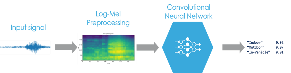
[오디오 파일의 전처리 및 CNN 학습 흐름도]

파이썬 버전에 따른 패키지들의 의존성이 상당히 민감하기 때문에 사용중인 운영체제의 안정성이 파괴되지 않도록 주의해야 합니다. 그래서 파이썬 소프트웨어를 다룰 때는, 가급적 Conda와 같은 파이썬 패키지의 가상화 환경 프로그램을 활용하는 것을 추천하고 싶습니다. 파이썬 패키지 설치는 pip install {package-name} 수행하도록 합니다. 만약, 이미 설치된 파이썬 패키지가 있다면, pip install --upgrade {package-name} 를 수행하여 패키지 버전을 업그레이드합니다.

import os

import numpy as np

from tqdm import tqdm

import matplotlib.pyplot as plt

from sklearn.model_selection import train_test_split

from sklearn import preprocessing

from sklearn.metrics import confusion_matrix

from sklearn.metrics import accuracy_score

import keras

from keras import layers

from keras import models

from keras import optimizers

# import tensorflow as tf

import tensorflow.compat.v1 as tf

#To make tf 2.0 compatible with tf1.0 code, we disable the tf2.0 functionalities

tf.disable_eager_execution()

import librosa.display

import librosa.util

이 프로젝트를 수행하기 위하여 사용된 Keras, TensorFlow, Librosa 패키지들의 버전정보는 다음과 같습니다. 이때 여기서 Keras는 딥러닝 프론트 엔드가 되고, TensorFlow은 딥러닝 백엔드의 역할을 수행합니다.

print("Python:", python.__version__)

print("Keras:", keras.__version__)

print("TensorFlow:",tf.__version__)

print("librosa:",librosa.__version__)

Keras (expected version: 2.2.4):  2.2.4

TensorFlow (expected version: 1.14.0):  1.14.0

librosa (expected version: 0.9.2):  0.9.2

IoT보드 준비

본 프로젝트를 수행하기 위하여 IOT보드에 마이크 장치가 포함되어 있어야 한다. 마이크 장치는 사용자 레벨의 애플리케이션 수준에서 녹음이 가능할 수 있도록 디바이스 드라이버와 저 수준의 시스템콜 라이브러리가 지원되어야 합니다.

다음은 B-L475E-IOT01A 보드의 하드웨어 스펙을 보여줍니다. 저는 해당 IOT보드가 마이크 기능을 (MP34D501) 지원하는지 데이터 시트 문서를 통하여 사전 체크해야 합니다. ST사의 "STM32F413RHT" Micom의 "DFSDM"기능이 Sigma-Delta입력 필터 기능을 수행을 하기 때문에 AMC1306칩의 출력인 Uncoded Bit stream형태의 신호를 MCU에서 받아서 내부 필터 기능을 적용하여 데이터화 합니다.

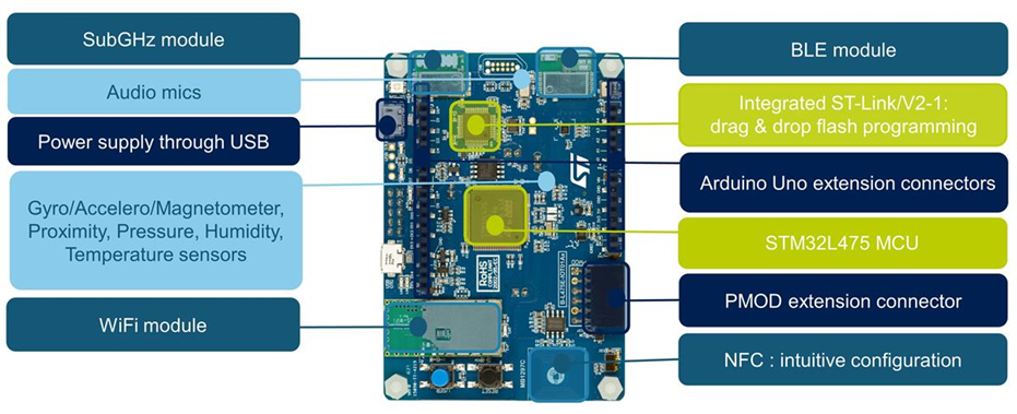
[B-L475E-IOT01A 개발보드의 하드웨어 정보]

오디오 데이터 생성

오디오 데이터 그룹 만들기

이 섹션은 오디오 데이터의 정보를 설명합니다. 실제 애플리케이션을 빌드하려면 완전한 데이터 세트를 사용하는 것이 좋습니다. 예를 들어, TUT Acoustic Scenes 2016 데이터셋을 (https://zenodo.org/record/45739#.YzjqqXblKUk) 사용할 수 있습니다. 각각의 데이터 세트는 다른 녹음 위치를 가진 다양한 음향 장면의 녹음으로 구성됩니다. 데이터 세트는 Dataset이라는 폴더 안에 위치시킵니다. 데이터세트에는 각 행에 오디오 파일에 대한 경로와 공백으로 구분된 레이블이 있는 메타데이터 파일을 다음과 같이 포함합니다.

bus.wav bus
park.wav park
home.wav home

원래 클래스(버스, 카페/레스토랑, 자동차, 등등)는 단순성을 위해 보다 일반적인 클래스(실내, 실외, 차량)로 집계됩니다. 런타임에 데이터가 로딩이 될 때, 샘플비율은16kHZ으로 재샘플링이 되고, 채널은 mono으로 변환됩니다.

주의) 오디오 신호 샘플링 속도 및 채널 번호 설정은 STM32 오디오 캡처 설정과 일치해야 합니다.

dataset_dir = './Dataset'

meta_path = path = os.path.join(dataset_dir, 'TrainSet.txt')

fileset = np.loadtxt(meta_path, dtype=str)

# 3 classes : 0 indoor, 1 outdoor, 2 in-vehicle

class_names = ['indoor', 'outdoor', 'vehicle']

labels = {

    'bus' : 2,

    'cafeRestaurant' : 0,

    'car' : 2,

    'cityCenter' : 1,

    'home' : 0,

    'office' : 0,

    'park' : 1,

    'residentialArea' : 1,

    'shoppingCenter' : 0,

    'subway' : 2,

    'train' :  2,

    'tramway' :  2,

x = []

y = []

for file in tqdm(fileset):

    file_path, file_label = file

    file_path = os.path.join(dataset_dir, file_path)

    # @note: resampling can take some time!

    signal, _ = librosa.load(file_path, sr=16000, mono=True, duration=30, dtype=np.float32)

    label = labels[file_label]

    x.append(signal)

    y.append(label)

100%|??????????| 3/3 [00:00<00:00, 106.86it/s]

plt.figure(figsize=(12, 2))

plt.title(class_names[y[0]])

librosa.display.waveshow(x[0], sr=16000)

plt.figure()

plt.plot(x[0])

plt.xlabel('Sample Index')

plt.ylabel('Amplitude')

plt.title('Waveform of Test Audio (Play)')

plt.show()

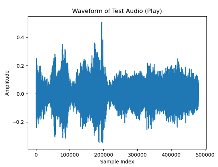
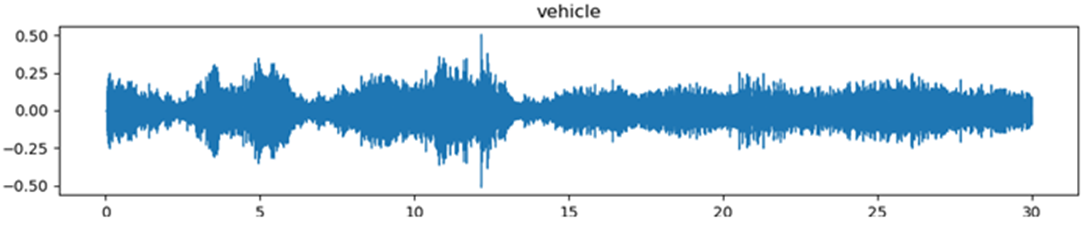
[주파스 레벨 측정 결과]

오디오 데이터 수집하기

일반적으로 사람의 귀는 소리를 비선형적으로 받아들입니다. 보통 청각의 감지 능력은 500Hz 이하의 소리에서는 1Hz의 변화도 구별을 할 수 있습니다. 그러나 2,000Hz 이상에서는 5Hz정도의 변화를 감지할 수 있다고 합니다. 즉 낮은 주파수에서는 작은 변화에도 민감하지만, 높은 주파수로 갈수록 민감도가 작아집니다. 이러한 청각의 특성을 반영하여 주파수 성분을 얻는 모델을 Mel Spectrogram이라고 합니다.

원래의 오디오 데이터를 신경망 모델에 제공하는 대신에 저는 LogMel Spectrogram이라는 '피쳐 (Feature)' 세트를 생성하기 위해 먼저 데이터를 더 작은 서브프레임으로 슬라이싱을 수행해야 합니다. 이러한 기능은 모델 학습, 검증 및 테스트에 사용되기 위한 것입니다.

Data를 (.wav) 생성하기

IoT개발보드의 마이크기능을 이용하여 .wav 포맷의 오디오 파일을 녹음을 합니다.

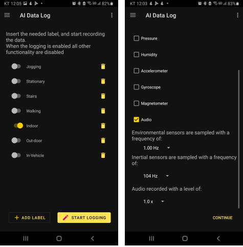
수집된 오디오 파일은 IOT 개발보드의 사용자 공간 (8MB)에 저장이 된다. IOT 개발보드의 USB 저장장치로부터 녹음한 오디오 파일을 가져오는 방법은 다음과 같습니다.

1단계, IOT 개발보드 뒷면의 JP4 점퍼선을 중간으로 (5~6)으로 다시 꼽습니다.
2단계, OT 개발보드의 STLink 포트가 아닌 USB OTG 포트에 USB 케이블을 연결합니다.
3단계, RESET 버턴을 누른 상태에서 USER 버턴을 눌려서 IOT 개발보드를 부팅합니다.
4단계, 다음과 같이 ST IOT 보드의 저장 장치에 보관된 IoT01****.wav 파일을 Host PC로 가져옵니다.

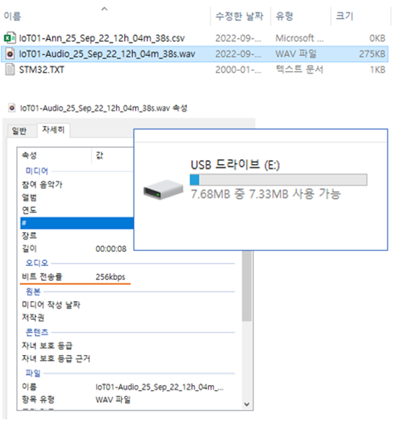
[ST IOT 개발보드에 저장한 wave 파일의 오디오 속성 정보]

다음 그림은 30초짜리, 256kbps 비트 전송률로 생성된 3타입의 .wav 파일을 보여주고 있습니다. 아래의 예처럼 각 wav 파일들을 30초 짜리 파일들을 녹화하도록 합니다.

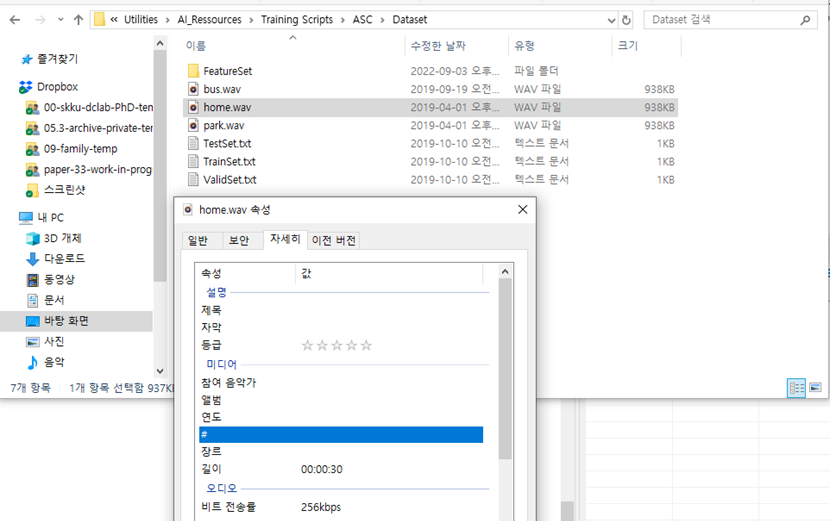
[Host PC의 “Dataset”폴더에 옮겨놓은 wave 파일 정보 내역]

Data로 LogMel Spectrogram 생성

각 프레임에는 16,896개의 샘플 (=32 x 512 + 512)이 포함됩니다. 그리고 다음 예제 코드에서 보여주는 것처럼, n_fft=1024 및 hop_length=512인 32열의 Spectrogram을 생성합니다.

x_framed = []

y_framed = []

for i in range(len(x)):

    frames = librosa.util.frame(x[i], frame_length=16896, hop_length=512)

    x_framed.append(np.transpose(frames))

    y_framed.append(np.full(frames.shape[1], y[i]))

# merge sliced frames and label

x_framed = np.asarray(x_framed)

y_framed = np.asarray(y_framed)

x_framed = x_framed.reshape(x_framed.shape[0]*x_framed.shape[1], x_framed.shape[2])

y_framed = y_framed.reshape(y_framed.shape[0]*y_framed.shape[1], )

print("x_framed shape: ", x_framed.shape) # Each frame of 16,896 samples can be used to create spectrogram

print("y_framed shape: ", y_framed.shape) # Corresponding label for each frame

x_framed shape:  (2715, 16896)

y_framed shape:  (2715,)

LogMel Spectrogram으로 전처리 작업

LogMel Spectrogram 특징점을 추출해야 합니다. 이 추출방법을 사용하여 특징 세트를 생성합니다. 이때 파이썬의 tqdm 함수를 이용하면 진척되는 현황을 모니터링할 때 편리합니다.

중요: 전처리 매개변수는 STM32 구현에 정의된 parameter와 일치해야 합니다.

x_features = []

y_features = y_framed

for frame in tqdm(x_framed):

    # Create a mel-scaled spectrogram

    S_mel = librosa.feature.melspectrogram(y=frame, sr=16000, n_mels=30, n_fft=1024, hop_length=512, center=False)

    # Scale according to reference power

    S_mel = S_mel / S_mel.max()

    # Convert to dB

    S_log_mel = librosa.power_to_db(S_mel, top_db=80.0)

    x_features.append(S_log_mel)

# Convert into numpy array

x_features = np.asarray(x_features)

100%|??????????| 2715/2715 [00:12<00:00, 218.58it/s]

특징점을 추출한 피쳐세트은 2,715개의 기능이 있습니다. 각 기능은 30 x 32크기의 Spectrogram으로 표시됩니다.

print(x_features.shape)

(2715, 30, 32)

다음 파이썬 코드는 피쳐 클래스를 위해 생성되는 Spectrogram을 그래프로 그리는 예제입니다. Plot 파이썬 모듈을 이용하여 그래프로 그리는 작업을 보여줍니다.

# Plot the first spectrogram generated for each feature class

plt.figure(figsize=(10, 8))

plt.subplot(311)

indoor_index = np.argmax(y_framed == 0)

librosa.display.specshow(x_features[indoor_index], sr=16000, y_axis='mel', fmax=8000,

                         x_axis='time', cmap='viridis', vmin=-80.0)

plt.colorbar(format='%+2.0f dB')

plt.title('LogMel spectrogram for ' + class_names[y_features[indoor_index]])

plt.subplot(312)

outdoor_index = np.argmax(y_framed == 1)

librosa.display.specshow(x_features[outdoor_index], sr=16000, y_axis='mel', fmax=8000,

                         x_axis='time', cmap='viridis', vmin=-80.0)

plt.colorbar(format='%+2.0f dB')

plt.title('LogMel spectrogram for ' + class_names[y_features[outdoor_index]])

plt.subplot(313)

vehicle_index = np.argmax(y_framed == 2)

librosa.display.specshow(x_features[vehicle_index], sr=16000, y_axis='mel', fmax=8000,

                         x_axis='time', cmap='viridis', vmin=-80.0)

plt.colorbar(format='%+2.0f dB')

plt.title('LogMel spectrogram for ' + class_names[y_features[vehicle_index]])

plt.tight_layout()

plt.show()

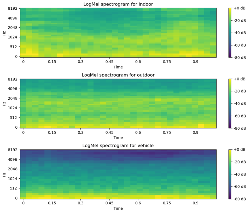
[3개로 분리한 클래스별 LogMel Spectrogram 정보 그래프]

피쳐 표준화하기

이제 평균을 제거하고 단위 분산에 맞게 조정하는 작업을 수행합니다. 피쳐 표준화를 위한 샘플 x의 표준 점수는 다음과 같이 계산합니다.

z = (x - u) / s

x: 샘플 값

u: 훈련 샘플의 평균

s: 훈련 샘플의 표준 편차

z: 표준화 점수

다음과 같이 스케일링을 위하여 피쳐들을 재구성을 합니다. 이때 피쳐 스케일러로 피쳐 변형을 수행합니다.

# https://scikit-learn.org/stable/auto_examples/preprocessing/plot_scaling_importance.html

# Flatten features for scaling

x_features_r = np.reshape(x_features, (len(x_features), 30 * 32))

# Create a feature scaler

scaler = preprocessing.StandardScaler().fit(x_features_r)

# Apply the feature scaler

x_features_s = scaler.transform(x_features_r)

데이터 인코딩하기

각 피쳐에는 각각 일치하는 레이블이 있습니다. 그러나 Keras에는 범용적인 One-Hot 인코딩 대상의 레이블 데이터가 필요합니다. 따라서, 레이블을 원하는 인코딩으로 변환해 보겠습니다.

# Convert labels to categorical one-hot encoding

y_features_cat = keras.utils.to_categorical(y_features, num_classes=len(class_names))

print("y_features_cat shape: " ,y_features_cat.shape)

y_features_cat shape:  (2715, 3)

데이터셋을 훈련, 검증, 테스트 셋으로 분리

저는 훈련할 때 이전에 본 적이 없는 데이터에 대한 모델의 정확도를 확인합니다. 그래서, 저는 데이터 세트를 훈련 및 검증 세트로 분할하여 각 훈련 Epoch이 끝날 때 손실 및 기타 모델 메트릭을 평가하기를 원합니다. 이 작업의 목표는 훈련 및 검증 데이터만 사용하여 모델을 개발하고 조정하는 것입니다. 테스트 세트는 알려지지 않은 새 데이터인 것처럼 최종 평가에만 사용됩니다.

# how to traing models with skleran

# https://scikit-learn.org/stable/modules/generated/sklearn.model_selection.train_test_split.html#sklearn.model_selection.train_test_split

x_train, x_test, y_train, y_test = train_test_split(x_features_s, y_features_cat, test_size=0.25, random_state=1)

x_train, x_val, y_train, y_val = train_test_split(x_train, y_train, test_size=0.25, random_state=1)

print('Training samples:', x_train.shape)

print('Validation samples:', x_val.shape)

print('Test samples:', x_test.shape)

Training samples: (1527, 960)

Validation samples: (509, 960)

Test samples: (679, 960)

(선택사항) 피쳐 저장하기

마지막으로 X-CUBE-AI가 이해할 수 있는 형식으로 피쳐들을 .csv 파일 포맷으로 저장합니다. 각 텐서에 대해 값이 평평한 벡터에 있습니다.

out_dir = './Output/'

np.savetxt(out_dir + 'x_train.csv', x_train.reshape(len(x_train), 30 * 32), delimiter=",")

np.savetxt(out_dir + 'y_train.csv', y_train, delimiter=",")

np.savetxt(out_dir + 'x_val.csv', x_val.reshape(len(x_val), 30 * 32), delimiter=",")

np.savetxt(out_dir + 'y_val.csv', y_val, delimiter=",")

np.savetxt(out_dir + 'x_test.csv', x_test.reshape(len(x_test), 30 * 32), delimiter=",")

np.savetxt(out_dir + 'y_test.csv', y_test, delimiter=",")

AI 모델 학습

이제 AI 모들을 생성하기 위하여 학습하고 평가하는 작업을 수행할 차례입니다.

AI 모델 그래프 만들기

이제 CNN 분류기 모델을 구축할 차례입니다. model.add 파이썬 함수를 이용하여 각 레이어별로 수행하고자 하는 내용들을 선언해주도록 합니다.

model = models.Sequential()

model.add(layers.Conv2D(16, (3, 3), activation='relu', input_shape=(30, 32, 1), data_format='channels_last'))

model.add(layers.MaxPooling2D((2, 2)))

model.add(layers.Conv2D(16, (3, 3), activation='relu'))

model.add(layers.MaxPooling2D((2, 2)))

model.add(layers.Flatten())

model.add(layers.Dense(9, activation='relu'))

model.add(layers.Dense(3, activation='softmax'))

# print model summary

model.summary()

WARNING: Logging before flag parsing goes to stderr.

The name tf.get_default_graph is deprecated. Please use tf.compat.v1.get_default_graph instead.

Please use tf.compat.v1.placeholder instead.

The name tf.random_uniform is deprecated. Please use tf.random.uniform instead.

The name tf.nn.max_pool is deprecated. Please use tf.nn.max_pool2d instead.

Layer (type)                 Output Shape              Param #

===============================================

conv2d_1 (Conv2D)            (None, 28, 30, 16)        160

_________________________________________________________________

max_pooling2d_1 (MaxPooling2 (None, 14, 15, 16)        0

_________________________________________________________________

conv2d_2 (Conv2D)            (None, 12, 13, 16)        2320

_________________________________________________________________

max_pooling2d_2 (MaxPooling2 (None, 6, 6, 16)          0

_________________________________________________________________

flatten_1 (Flatten)          (None, 576)               0

_________________________________________________________________

dense_1 (Dense)              (None, 9)                 5193

_________________________________________________________________

dense_2 (Dense)              (None, 3)                 30

==============================================

Total params: 7,703

Trainable params: 7,703

Non-trainable params: 0

AI 모델 빌드하기

Loss Function을 계산할 때 전체 Train-Set을 사용하는 것을 Batch Gradient Descent라고 합니다. 그러나 이렇게 계산하면 한번 step을 내딛을 때마다 전체 데이터에 대해 Loss Function을 계산해야 합니다. 이렇게 되면 너무 많은 계산양을 필요로 합니다. 이를 방지하기 위해 Stochastic Gradient Descent (SGD)라는 방법을 사용합니다. 따라서, Loss Function을 계산할 때, 전체 데이터(Batch) 대신 일부 데이터의 모음(Mini-Batch)를 사용하여 Loss Function을 계산합니다. Batch Gradient Descent보다 다소 부정확할 수는 있지만, 계산 속도가 훨씬 빠르기 때문에 같은 시간에 더 많은 step을 갈 수 있습니다. 그 다음 AI 모델을 최종적으로 빌드하는 작업을 수행하도록 합니다.

sgd = optimizers.SGD(lr=0.01, momentum=0.9, nesterov=True)

model.compile(optimizer=sgd, loss='categorical_crossentropy',  metrics=['acc'])

The name tf.train.Optimizer is deprecated. Please use tf.compat.v1.train.Optimizer instead.

The name tf.log is deprecated. Please use tf.math.log instead.

AI 모델 훈련하기

이제 훈련 데이터를 모델에 입력할 차례입니다. 이 작업에는 많은 시간이 소요되기 때문에 고성능의 CPU 또는 GPU가 권장됩니다.

# Reshape features to include channel

x_train_r = x_train.reshape(x_train.shape[0], 30, 32, 1)

x_val_r = x_val.reshape(x_val.shape[0], 30, 32, 1)

x_test_r = x_test.reshape(x_test.shape[0], 30, 32, 1)

AI 모델을 학습하기 위하여 다음과 같이 model.fit 함수를 이용하여 지정된 epoch 횟수만큼 학습을 수행하도록 합니다.

# Train the model

history = model.fit(x_train_r, y_train, validation_data=(x_val_r, y_val),

                    batch_size=500, epochs=30, verbose=2)

Epoch 1/10

2022-10-01 15:36:08.448797: I tensorflow/core/platform/cpu_feature_guard.cc:142] Your CPU supports 
instructions that this TensorFlow binary was not compiled to use: AVX

 - 1s - loss: 1.1662 - acc: 0.1657 - val_loss: 1.0465 - val_acc: 0.6326

Epoch 2/10

 - 1s - loss: 1.0344 - acc: 0.6385 - val_loss: 0.9907 - val_acc: 0.6483

Epoch 3/10

 - 1s - loss: 0.9668 - acc: 0.6483 - val_loss: 0.8680 - val_acc: 0.6582

Epoch 4/10

 - 1s - loss: 0.8237 - acc: 0.6627 - val_loss: 0.6569 - val_acc: 0.6974

Epoch 5/10

 - 1s - loss: 0.6127 - acc: 0.7289 - val_loss: 0.4824 - val_acc: 0.8134

Epoch 6/10

 - 1s - loss: 0.4768 - acc: 0.8062 - val_loss: 0.3702 - val_acc: 0.9234

Epoch 7/10

 - 1s - loss: 0.3537 - acc: 0.9103 - val_loss: 0.2569 - val_acc: 0.9136

Epoch 8/10

 - 1s - loss: 0.2483 - acc: 0.9214 - val_loss: 0.1819 - val_acc: 0.9371

Epoch 9/10

 - 1s - loss: 0.1824 - acc: 0.9325 - val_loss: 0.1489 - val_acc: 0.9430

Epoch 10/10

 - 1s - loss: 0.1499 - acc: 0.9371 - val_loss: 0.1206 - val_acc: 0.9528

Evaluate model:

                         ……… Omission ………

 32/679 [>.............................] - ETA: 0s

352/679 [==============>...............] - ETA: 0s

672/679 [============================>.] - ETA: 0s

679/679 [==============================] - 0s 174us/step

[0.12382532915152576, 0.9587628865979382]

Test loss: 0.123825

Test accuracy: 95.88%

Accuracy = 95.88%

이제 학습된 AI 모델의 손실 현황 추이를 살펴보기 위하여 다음과 같이 시각화된 그래프로 출력합니다.

train_loss = history.history['loss']

val_loss = history.history['val_loss']

plt.figure()

plt.clf()

plt.xlabel('Epochs')

plt.ylabel('Loss')

plt.plot(train_loss, color='r', label='training loss')

plt.plot(val_loss, color='g', label='validation loss')

plt.legend()

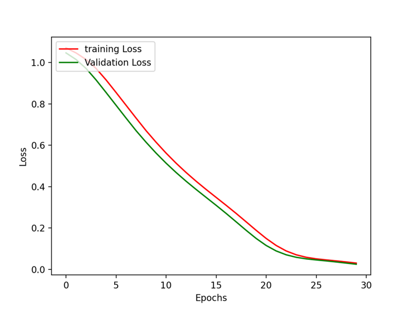
[학습 및 검증의 epoch 별 손실율 변화 그래프]

Accuracy 평가하기

다음으로, 모델이 테스트 데이터 세트에서 수행하는 방식을 비교합니다.

print('Evaluate model:')

results = model.evaluate(x_test_r, y_test)

print(results)

print('Test loss: {:f}'.format(results[0]))

print('Test accuracy: {:.2f}%'.format(results[1] * 100))

Evaluate model:

679/679 [==============================] - ETA:  - ETA:  - ETA:  - ETA:  - 0s 292us/step

[0.0033203214310954525, 1.0]

Test loss: 0.003320

Test accuracy: 100.00%

Overfitting (과적합) 은 머신 러닝 모델이 훈련 데이터보다 새로운 데이터에서 더 나쁜 성능을 보이는 경우입니다.

Confusion Matrix 평가하기

혼돈행렬 (Confusion Matrix)은 학습을 통한 Prediction 성능을 측정하기 위한 것입니다. Prediction value와 Actual value를 비교하기 위한 표입니다.

y_pred = model.predict(x_test_r)

y_pred_class_nb = np.argmax(y_pred, axis=1)

y_true_class_nb = np.argmax(y_test, axis=1)

accuracy = accuracy_score(y_true_class_nb, y_pred_class_nb)

np.set_printoptions(precision=2)

print("Accuracy = {:.2f}%".format(accuracy * 100))

cm = confusion_matrix(y_true_class_nb, y_pred_class_nb, labels=[0,1,2])

# (optional) normalize to get values in %

# cm = cm.astype('float') / cm.sum(axis=1)[:, np.newaxis]

# Loop over data dimensions and create text annotations.

thresh = cm.max() / 2.

for i in range(cm.shape[0]):

    for j in range(cm.shape[1]):

        plt.text(j, i, format(cm[i, j], 'd'),

                ha="center", va="center",

                color="white" if cm[i, j] > thresh else "black")

plt.imshow(cm, cmap=plt.cm.Blues)

Accuracy = 100.00%

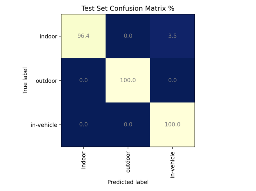
[Counfusion Matrix 의 그래프 출력 결과]

생성한 AI 모델 저장

딥러닝 환경에 훈련한 AI모델을 저장할 때, 일반적으로 파일 확장자는 .ckpt, .pb, .h5 등의 3개의 포맷이 범용적입니다. 각각의 파일 포맷의 주요 차이는 다음과 같습니다.

ckpt: Pytorch에 주로 사용되는 포맷이다. 그래프 (=모델구조)만 있는 .ckpt-meta 파일, 가중치(weight)만 있는 .ckpt-data 파일로 구성된다.
pb: 모델구조 (graph)와 가중치 (weight) 를 모두 가지고 있는 파일이다.
h5: Keras에서 주로 사용하는 포맷이다. 그래프 (=모델구조)와 가중치(weight)를 모두 가지고 있는 파일이다.

이제 학습한 AI 모델을 .h5 파일 형식으로 저장하기 위하여 model.save( )명령을 수행합니다.

# Save the model into an HDF5 file ‘model.h5’

model.save(out_dir + 'model.h5')

(선택사항) 양자화로 TFLite 모델 변환

TensorFlow Lite 변환기를 사용하여 추가적인 최적화를 수행할 수 있습니다. 일반적으로 TensorFlow Lite 변환기는 CPU 및 DRAM 메모리 용량이 제한적인 임베디드 장치들을 지원하기 위하여 정확도를 희생시키는 대신에 모델 크기가 줄이는 기능을 도모합니다. 본 작업을 위하여 아래의 사이트를 참고하여 양자화하는 방법에 대한 도움을 받았습니다.

x_train_r.shape

(1527, 30, 32, 1)

def representative_dataset_gen():

    for i in range(len(x_train_r)):

        yield [x_train_r[i].reshape((1, ) + x_train_r[i].shape)]

converter = tf.lite.TFLiteConverter.from_keras_model_file(out_dir + "model.h5" )

converter.optimizations = [tf.lite.Optimize.DEFAULT]

converter.representative_dataset = representative_dataset_gen

converter.target_ops = [tf.lite.OpsSet.TFLITE_BUILTINS_INT8]

converter.inference_input_type = tf.int8

converter.inference_output_type = tf.int8

tflite_model = converter.convert()

with open(out_dir + 'model.tflite','wb') as f:

    f.write(tflite_model)

    print("TFlite model saved")

W1024 11:46:57.122369 437772 deprecation.py:323] From c:\users\chiphead\appdata\local\programs\python
\python36\lib\site-packages\tensorflow\lite\python\util.py:238: convert_variables_to_constants 
(from tensorflow.python.framework.graph_util_impl) is deprecated and will be removed in a future version.

Instructions for updating:

Use `tf.compat.v1.graph_util.convert_variables_to_constants`

W1024 11:46:57.125878 437772 deprecation.py:323] From c:\users\chiphead\appdata\local\programs\python
\python36\lib\site-packages\tensorflow\python\framework\graph_util_impl.py:270: extract_sub_graph 
(from tensorflow.python.framework.graph_util_impl) is deprecated and will be removed in a future version.

Instructions for updating:

Use `tf.compat.v1.graph_util.extract_sub_graph`

TFlite model saved

STM32.XCube AI 툴

생성된 AI 모델을 IOT 개발보드에 실행가능한 C 소스코드로 변환합니다. 그리고 C소스코드를 빌드하는 작업을 하는 방법을 설명합니다.

AI 모델을 C코드로 변환

XCube.MX 도구는 사전 훈련된 모델 .h5 파일을 로딩후, STM32 IOT 개발 장치를 위한 최적화된 C 언어 기반의 모델을 생성할 수 있습니다. XCube.MX 도구를 실행하면 생성되는 asc.*, asc_data.* 파일들을 STM32CubeFunctionPack_SENSING1_V4.0.3의 소스 폴더에 복사 및 붙여넣기를 하도록 합니다.

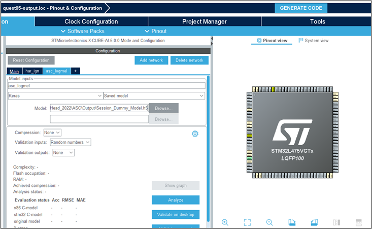
[STM32 Cube MX을 이용하여 .h5를 C코드로 변환하는 예시]

C 소스코드의 빌드 및 플래싱

STM32Cube IDE를 이용하여 생성한 ASC C소스코드를 빌드하여 펌웨어 이미지를 생성한다. 그리고나서 생성한 펌웨어 이미지를 IOT 개발보드에 플래싱을 수행하도록 한다.

[MCU GCC 컴파일러: C/C++ 소스코드의 빌드 옵션]

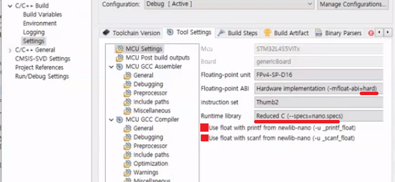
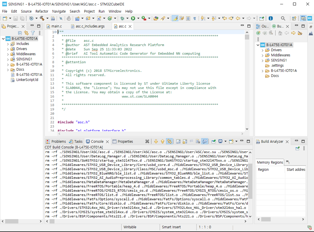
[STM32 Cube IDE을 이용하여 C 소스 생셩 결과 예제]

데모

오디오 분류 페이지는 FP-AI-SENSING1과 함께 제공되는 ASC 알고리즘의 AI 신경망 분류 결과를 모니터링하는 데 사용할 수 있으며, 다음 인식된 오디오 장면 중 하나를 알릴 수 있습니다.

• Indoor
• Outdoor
• In-Vehicle

[음향 소리 인식: 초기화] [음향 소리 인식: Home] [음향 소리 인식: Mic Plot Data]

STM32Cube MX의 ASC 모델의 모델구조(=Graph)와 가중치 (=Weight)를 분석합니다. AI 모델의 전체 레이어는 다음 그림에서 보여주는 바와 같이 컨볼류션 및 풀링을 통해 반복 학습을 수행하였고, 이렇게 학습한 내용들을 최종 레이어에서 Fully Connected Layer으로 구성하기 위하여 Dense 오퍼레이션을 수행하였습니다.

[모델구조 세부 구조도]

다음 그림을 학습한 가중치 데이터들을 참고 있는 weight 배열의 정보들을 보여주고 있습니다. ST IOT 개발보드의 RAM 용량에 맞는 만큼 적절히 배열 사이즈를 조절해주어야 합니다. 그렇지 않으면 C 소스코드를 빌드 하는 과정에서 “region `RAM' overflowed by 4240 bytes” 와 같은 에러 메시지를 만나게 됩니다.

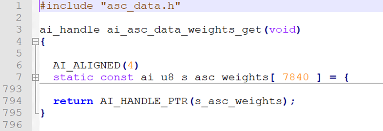
[가중치 정보]

* 데모: B-L475E-IOT01A 보드에서 구동하는 동영상

음향 장면 인식 기술은 시각적으로 확인할 수 없는 사각지대에 발생한 예상치 못한 상황을 소리만으로도 인식할 수 있습니다. 딥러닝 기술을 이용하여 IoT 장치의 마이크가 캡처한 주변 소음을 더 세밀하게 분류할 수 있습니다. 이번 프로젝트에서는 ST MicroElectronics사의 IoT 개발보드에 내장되어 있는 마이크 장치를 이용하여 음향을 입력받고, 학습후 AI모델을 만들었습니다. 그다음, 생성한 AI모델을 C 소스 코드로 변환하고, 컴파일하여 펌웨어 이미지를 만들고, 이 펌웨어 이미지를 개발보드에 플래싱합니다. 최종적으로 입력되는 음향을 분석함으로써, Indoor 음성인지, Outdoor 음성인지, In-Vehicle 음성인지 분류해내는 CNN 기반 딥러닝 소프트웨어를 데모합니다.